A Guide to SPICE Simulation in Altium NEXUS

Introduction

A circuit is a set of components connected together to deliver the functionality and performance that your product requires. The parameters of the components you need in the circuit can be determined by:

1. Manual mathematical calculations.
2. Сreating a prototype of the actual design, and then testing it.
3. Computer-based mathematical simulation, aka SPICE.

The most efficient and cost-effective option is the use of modern methods of mathematical simulation, using Computer-Aided Design (CAD) systems.

Modern electrical circuit CAD systems combine the ability to simulate circuits that include both analog and digital devices. The use of computer simulation makes it possible to experiment, obtain real circuit characteristics, evaluate possible risks in the device, and also achieve the implementation that best delivers the product's intended operational range and characteristics.

This guide covers the basic principles of SPICE simulation, how to avoid mistakes, as well as lots of information on learning how to use the tool.

Simulation, what is it and why is it necessary?

The main purpose of simulating the function of an electronic device is to represent and analyze the performance of the design. The jump from experimental methods to computer software simulation happened quite a long time ago. However, it is impossible to imagine the design of even the simplest device without the capabilities that simulation offers.

The use of a simulation program makes it possible to analyze all modes of the device being designed without possible damage, to determine parameters and characteristics that are difficult to measure in real conditions, and to perform measurements that might otherwise require the use of expensive measurement equipment. And the results of these simulations can conveniently be grouped on one plot, they can use several axes, you can change the display color, take measurements directly from the plots, share the results with colleagues, and much more.

SPICE (Simulation Program with Integrated Circuit Emphasis) was developed as an open-source software package, which has led to its broad popularity and continued development. Altium's Mixed Simulation (MixedSim) technology uses an improved core based on SPICE algorithms and is designed to simulate analog, digital or mixed analog-to-digital device electrical circuits.

This guide will cover not only the mechanisms for obtaining basic circuit characteristics, but also the features of circuit design for simulation, the process of adding models to circuit elements, and the description of the Netlist document and its application.

What can we Simulate using SPICE?

Altium's simulation technology is under active development, including the variety of supported models and model types (including Pspice & LTSpice), the underlying algorithms, and the available types of circuit analyses.

The simulator supports the following types of analyses:

• Operating Point - determines the dc operating point of a circuit, with inductors shorted and capacitors opened.
• Poles and Zeros of transfer function - used to determine the stability of a single input, single output linear system, by calculating the poles and/or zeros in the small-signal ac transfer function for the circuit. The dc operating point of the circuit is found and then linearized, small-signal models for all non-linear devices in the circuit are determined. This circuit is then used to find the poles and zeros that satisfy the nominated transfer function.
• DC Transfer function - (DC small signal analysis) calculates the DC input resistance, DC output resistance and DC gain, at each voltage node in the circuit.
• DC sweep - generates output like that of a curve tracer. Used to sweep variables, including: temperature, voltages and currents from sources, resistances and conductivity.
• Transient analysis - generates output similar to that normally shown on an oscilloscope, computing the transient output variables (voltage or current) as a function of time, over the user-specified time interval. An Operating Point analysis is automatically performed prior to a Transient analysis to determine the DC bias of the circuit, unless the Use Initial Conditions parameter is enabled.
• Fourier analysis - Fourier analysis of a design is based on the last cycle of transient data captured during a Transient analysis. For example, if the fundamental frequency is 1kHz, then the transient data from the last 1ms cycle would be used for the Fourier analysis.
• AC sweep - Linear or low-signal frequency response. Generates output that shows the frequency response of the circuit, calculating the small-signal AC output variables as a function of frequency. It first performs an Operating Point analysis to determine the DC bias of the circuit, replacing the signal source with a fixed amplitude sine wave generator, then analyzing the circuit over the specified frequency range. The desired output of an AC Small Signal analysis is usually a transfer function (voltage gain, transimpedance, etc).
• Noise analysis - measures the noise contributions of resistors and semiconductor devices by plotting the Noise Spectral Density, which is the noise measured in Volts squared per Hertz (V²/Hz). Capacitors, inductors, and controlled sources are treated as noise free.
• Temperature sweep - used to analyze the circuit at each temperature in a specified range, producing a series of curves, one for each temperature setting. The Simulator performs multiple passes of any of the standard analyses that are enabled (AC, DC Sweep, Operating Point, Transient, Transfer Function, Noise).
• Parameters sweep - used to sweep the value of a device in defined increments, over a specified range. The Simulator performs multiple passes of any of the standard analyses that are enabled (AC, DC Sweep, Operating Point, Transient, Transfer Function, Noise). The Parameter Sweep can vary basic components and models - subcircuit data is not varied during the analysis. You can also define a Secondary parameter to be swept, when a Secondary parameter is defined the Primary parameter is swept for each value of the Secondary parameter.
• Monte Carlo analysis - used to perform multiple simulation runs with component values randomly varied across specified tolerances. The Simulator performs multiple passes of any of the standard analyses that are enabled (AC, DC Sweep, Operating Point, Transient, Transfer Function, Noise). The Monte Carlo analysis can vary basic components and models - subcircuit data is not varied during the analysis.
• Sensitivity analysis - calculates sensitivities as numeric values of given measurements related to components/model parameters of circuit components, as well as sensitivity to temperature/global parameters. The result of the analysis is a table of the ranged values of sensitivities for each measurement type.

What are SPICE Models?

To simulate the performance of the devices in a design each component is represented in the form of a mathematical model, which is attached to the component as a SPICE model. The models do not fully represent the characteristics of the real components, they reflect their basic properties. Component models are the most important elements in the simulation process, since the data in the model determines the validity of the characteristics and reliability of the analysis.

The simulator supports popular SPICE-model formats, including the Altium MixedSim format (SPICE), as well as the widely used PSPICE and LTSPICE formats. Model files with the extensions .mdl, .ckt, .lib and .cir can be used.

The model (or macro model) is attached to the schematic symbol, either in the schematic library editor, or to the component once it has been placed on the schematic sheet. You can use the simulation-ready components in the installed Altium NEXUS libraries, or source models from many component manufacturers.

The software includes the following libraries that contain simulation-ready components (as shown in the image below):

• Simulation Generic Components - set of common components, including discretes, basic logic elements, pushbuttons, relays, sources, etc
• Simulation Math Function - set of mathematical functions
• Simulation Sources - set of current and voltage sources
• Simulation Pspice Functions - set of Pspice functions
• Simulation Special Function - set of special functions, including S-domain transfer functions; hysteresis, summer, differentiator and integrator blocks; and others
• Simulation Transmission Line - set of transmission lines
• Miscellaneous Devices (library of various elements, approx 75% of the components have a simulation model)

The available libraries and model files are installed and accessed through the Components panel.

Signal Sources

In order to simulate a circuit, a signal source is normally required to stimulate the circuit. The Simulation Generic Components and the Simulation Sources libraries include a large set of DC and AC current and voltage sources, controlled current and voltage sources, and signal sources of various types.

The Simulation Sources library includes the following elements:

• VSRC / ISRC - DC voltage / current source
• VSIN / ISIN - sinusoidal signal
• VPULSE / IPULSE - right-angle, trapezoidal or triangular shape, depending on the settings
• VEXP / IEXP - exponential waveform
• VPWL / IPWL - interpolated (piecewise linear) source
• VSFFM / ISFFM - frequency-modulated source
• BVSRC / BISRC - non-linear dependent source
• ESRC / GSRC - voltage / current source, controlled by voltage at the input pins
• HSRC / FSRC - voltage / current source, controlled by level of current flowing in the input pins
• .IC & .NS - elements to specify the initial conditions of the transient process
• DSEQ / DSEQ2 - data sequencer with clock output / data sequencer (the operation principle is a sequential reading of the state from the input file and setting this state on the outputs)

The Simulation Sources library contains a variety of sources.

Placing and Configuring a Source

As well as placing a source from a library, you can also use the Simulate » Place Sources menu in the schematic editor to place voltage and current sources on the schematic sheet.

Use the Source commands to place the required source on the schematic.

Sources can also be placed from the Active Bar, click and hold on the button to display the menu of special circuit elements. The last-used element will become the default for that button.

Alternatively, place sources using the Active Bar.

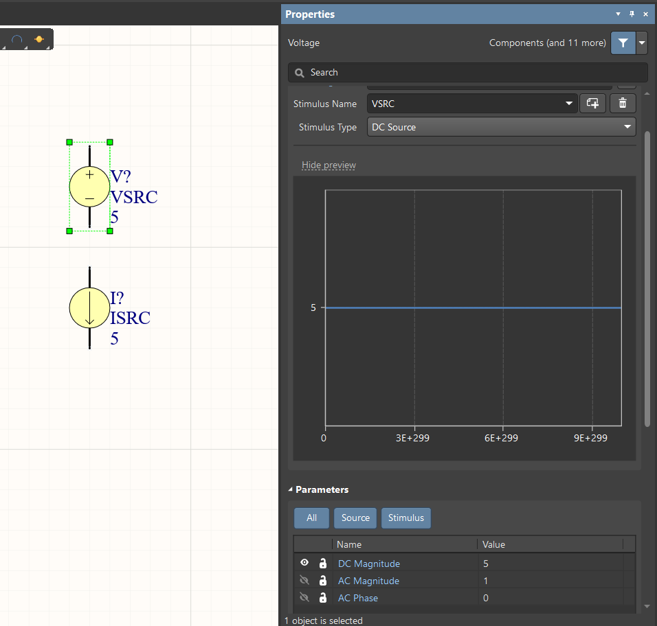
Once the source has been placed on the schematic, double-click on it to open the Properties panel. Note that you can change the Stimulus Type in the drop-down menu, when you do the set of parameters available to configure that source will automatically change.

Notes about working with sources:

• You can open the Properties panel by double-clicking on the selected element, or by clicking the Panels button () at the bottom right of the workspace.
• Enter a suitable name for the source in the Stimulus Name field. Note that this field remains unchanged when you change the source type, as it is a user-defined field. Note that if multiple sources share the same Stimulus Name, edits made to the properties of one source will also be applied to other sources with the same name.
• If you change the stimulus type, the graphic does not update. If this is an issue, place the source showing the required graphic directly from the library.
• The DC current or voltage values specified in the DC Magnitude parameter are used for DC circuit calculations, the AC Magnitude and AC Phase parameters are used for frequency calculations, and the Time functions are used to calculate the transient process for the current or voltage of the source.

The following parameters are set for DC voltage and current sources (as shown below):

• DC Magnitude
• AC Magnitude
• AC Phase

The set of parameters for sinusoidal voltage and current sources includes similar parameters for the DC and AC components, as well as the following elements (shown in the image below):

• Offset - the constant component of the signal (when using the Transient calculation)
• Amplitude
• Frequency
• Delay
• Damping Factor

The parameters of a sinusoidal signal source.

The Properties panel includes a preview window that shows the signal, based on the specified parameters. This allows you to track the changes you have made and verify their correctness. You can hide and display the preview window by clicking the Hide Preview / Show Preview link.

Use the preview window to verify that your settings are correct.

Each type of source has its own set of parameters that must be configured, for example, the VPULSE is shown below:

• Initial Value - initial value of the output signal
• Pulsed Value - pulse amplitude
• Time Delay – signal time delay
• Rise Time - signal rise time
• Fall Time - signal fall time
• Pulse Width - pulse width
• Period - period of signal

The set of parameters of a VPULSE source.

It is often necessary to create a complex piecewise linear signal when the waveform is specified by the user. In this situation, interpolated VPWL and IPWL voltage and current sources can be used. The signal parameters of these sources are set by creating suitable Time-Value Pairs. This row contains the coordinate values of the axes as a numerical sequence, as shown below.

The shape of the waveform is defined by the Time-Value pairs.

Configuring and Running a Simulation

MixedSim can be used to obtain a number of different characteristics of the electrical circuit in the form of tables and plots. The Simulation Dashboard is used to control the analysis, define the view and adjust parameters. You can open the Dashboard from the Simulate menu, or the Panels menu.

   Open the Simulation Dashboard to configure and control the simulation process.

The Schematics to Simulate

Before you start the simulation, you must choose which documents are to be included in the simulation. It can be just the active schematic sheet (Document), or the whole project (Project), consisting of several sheets. The selection is made at the top of the Simulation Dashboard from the Affect drop-down menu.

Define which schematic sheets are to be included in the simulation.

Circuit and Model Verification

As previously stated, the first step after creating a schematic is to verify the schematic and the component models. The verification process, along with examples of possible errors are described in more detail below, in the Schematic Design for Simulation section.

Preparing to Simulate

The next step is Preparation, where you confirm the Simulation Sources are correctly configured, and you can add Probes to measure voltage, current or power, at specific locations within the circuit.

Confirm that the Simulation Sources are correct and place any required Probes in the Preparation stage.

The image above shows the Preparation section of the Simulation Dashboard, displaying the Simulation Sources and Probes detected on the schematic. To demonstrate the different modes of calculation, the example above uses two constant voltage power sources (VSRC) and the simulation-ready pulse voltage source (VPULSE).

Each Source and Probe includes a checkbox, this can be used to temporarily disable that Source or Probe. This feature allows you to add multiple sources with different characteristics to the same point in the circuit, and then enable / disable them as you need when running different simulations.

Each Source and Probe also includes an button, when this is clicked that Source/Probe is deleted from the design - note that this action cannot be undone. Probes also include a color selector, as shown in the image below.

Additional probes can be placed by clicking the Add link, and the color can be user-configured.

Including Measurement Probes

Probes are used to take measurements at the location they are placed on the circuit. Probes can be used to track current, voltage, or power values and to display them on a plot. The display of the Probe name and value is configured in the Properties panel, each of these can be hidden or shown.

Configure the Name of the Probe and the display of the Value in the Properties panel (when the Probe is selected).

If the Probe is correctly connected, the designation is automatically assigned to the Probe. If the connection is incorrect, the text Empty Probe will be displayed instead of the designation, as shown below.

When a Probe is not correctly connected, it will display the text Empty Probe.

Analysis Setup & Run

The next step is to select the type of calculation, set the parameters, and Run the simulation.

The list of available calculation types includes:

• Calculation of operating points (Operating Point)
• Calculation in DC Sweep mode (DC Sweep), including voltage-current characteristics
• Transient process calculation (Transient) is a virtual oscilloscope
• Frequency analysis (AC Sweep), amplitude-frequency characteristic and phase-frequency characteristic

Available calculation types.

Operating Point Analysis

The Operating Point analysis calculates the values of current and voltage balance points in a steady-state circuit operation, the transfer coefficients in DC mode, as well as calculating the poles and zeros of the AC transfer characteristic that is required in other types of calculations.

Click Run to the right of the Operating Point text to perform an Operating Point analysis. A new document tab will automatically open, displaying the <ProjectName>.sdf file. The SDF document will include a single Operating Point tab (shown at the bottom of the workspace) that displays the calculations of all previously configured Probe points. Values are automatically calculated for all nodes in the circuit, these can be added to the results table by double-clicking on the Wave Name in the Sim Data panel when the SDF document is active.

Click Run to perform an Operating Point analysis (first image). The results are displayed in the SDF file that opens (second image).

You can also use the Display on schematic group of buttons to display the calculated values directly on the schematic. The values of voltages, power and currents can be displayed simultaneously and independently of each other, as shown below.

Display the calculated values directly on the schematic by clicking the required Display on schematic button(s).

The parameters of the additional Advanced calculations in this section are hidden. To enable the calculations and set the parameters, tick the appropriate checkboxes: Transfer Function and Pole-Zero Analysis, as shown in the image below.

• Transfer Function - is the calculation of transfer coefficients in DC mode, where the voltage source (Source Name) and the reference node of the circuit (Reference Node) must be defined.
• Pole-Zero Analysis - is the calculation of the poles and zeros of the AC transfer characteristic. For this calculation select the input and output signal nodes (Input Node / Output Node), input and output reference nodes (Input Reference Node / Output Reference Node), calculation type (Analysis Type) and type of function to be calculated (Transfer Function Type) from the drop-down menus.

Once the settings have been configured, click the  button to perform the analysis.

Configure the setting parameters for the additional calculations.

DC Sweep

Calculations performed in the DC mode allow you to see what happens in the circuit as you change the values of sources and resistors.

You set the parameters and output expressions and start the calculation in the DC Sweep section. Click the +Add Parameter link to add the source(s) to be analyzed. In the From / To / Step fields you must specify the initial value of the source range, the final value, and the step size.

Setting parameters and output expressions in the DC Sweep mode.

Additional output expressions (except active probes) can be added in the Output Expression section by clicking the +Add link. When an empty row appears, specify the output expression. This can be done manually, or you can click the button and select from the list of available Waveforms in the Add Output Expression dialog. Here you can not only select the desired signal from the list, but also define a mathematical expression using the menu of functions.

You also configure how those results should be plotted in the Add Output Expression dialog. In the Name and Units fields, you can specify the name of the output expression and the unit of measurement. Configure the Plot Number and Axis Number dropdowns to add the expression to an existing Plot / Axis, or create new ones.

Once the settings have been configured, click the  button to perform the analysis.

Select the required output expression or define a new function, then configure how that expression is to be plotted.

When the DC Sweep analysis is run, the results will display on a tab in the SDF document labeled DC Sweep. The upper Plot in the image below shows the DC Sweep results, displaying the current characteristics on the pins of the resistor R7 (shown in the previous schematic example image). The lower Plot shows the voltage source values V3 before and after passing through the circuit.

An example of a DC Sweep calculation.

Transient

The Transient analysis calculates the signal as a function of time. The time period can be defined as an Interval of time or as a number of cycles (Periods), by clicking the required mode button .

• Interval mode - select the Interval mode (), then define the From / To / Step values (initial time value / final time value / time step).
• Period mode - select the Period mode () - then define the From / N Periods / Points/Period values (initial value / number of periods to display / number of points per period).

Additional output expressions (except active probes) can be added in the Output Expression section by clicking the +Add link. When an empty row appears, specify the output expression. This can be done manually, or you can click the button and select from the list of available Waveforms in the Add Output Expression dialog. Here you can not only select the desired signal from the list, but also define a mathematical expression using the menu of functions.

Once the settings have been configured, click the  button to perform the analysis.

Settings for a transient calculation.

Fourier Analysis

The Fourier analysis, i.e. spectral analysis, is a method of analyzing periodic waveforms. It can be performed as an additional option when performing a transient analysis. To perform a Fourier analysis, enable this option and set the Fundamental Frequency and the Number of Harmonics.

The Use Initial Conditions checkbox allows you to use initial conditions to calculate the transient process.

Once the settings have been configured, click the  button to perform the analysis.

Configure the parameters of the Fourier Analysis.

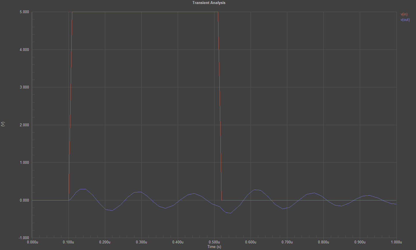
The results of the calculation are shown in a separate Transient Analysis tab in the SDF document, with a representation in the time domain of the output signal from the source (at the point in) and the output signal (at the point out.

Transient Analysis tab showing the Fourier analysis calculation results.

AC Sweep

The AC Sweep calculation is used to determine the frequency response of the system, that is, the dependence of the output signal amplitude on the input signal frequency.

Before performing the calculation, specify the values of the Start Frequency / End Frequency, and the number of points (No. Points, Points/Decade, or Points/Octave) for the distribution type selected in the Type dropdown. The method of selecting the output expressions is similar to the previous types of analysis.

Set parameters for the AC Sweep calculation.

Note that for an AC Sweep analysis, you can select from a range of Complex Functions, selected in the Add Output Expression dialog.

Selecting a Complex function for an AC Sweep analysis.

Noise Analysis

The AC Sweep includes an optional Noise Analysis. Noise calculation parameters are hidden by default, they become visible once a Noise Analysis has been enabled.

• Noise Source – source that is injecting noise into the circuit
• Output Node – node that the noise is being calculated for
• Ref Node – node that the noise analysis is referenced from
• Points Per Summary – the frequency of the noise of each device that generates noise

Noise Analysis parameters.

The result of the calculation is the graphical display of the dependence of the output signal amplitude on the input signal frequency in a separate AC Sweep tab.

AC Sweep calculation results.

Additional Analyses

At the bottom of the Analysis Setup & Run section are options for varying the parameters of the different calculation types. The principle of additional calculations is based on going through the values of the parameters within the selected range and executing a series of calculations for each value of the parameters. You can enable each of the additional calculations by ticking the required checkbox.

Enable additional calculations at the bottom of the Analysis Setup & Run section.

The settings for the additional calculations are configured in the Advanced Analysis Settings dialog, click the button to open the dialog.

Parameters for additional calculations.

Temperature Sweep

For the Temperature Sweep mode, the variable parameter is temperature. To simulate the behavior of the circuit at different temperatures, enable the Temperature checkbox and define (in degrees Celcius), the From (initial temperature), To (final temperature) values of the range, and the temperature Step size.

Parameters for the Temperature Sweep mode.

As an example, we can use the temperature sweep to calculate the current values on the R7 resistor pins using the Operating Point mode (first image below) and DC Sweep (second image below).

Results of Operating Point calculation using the temperature enumeration.

Results of the DC Sweep calculation with the Temperature Sweep enabled.

Selection of the output waveform for parametric calculations.

Sweep Parameter

The parameter that is enumerated in Sweep Parameter mode is the basic parameter that the component has; for example, the resistance value for resistors, capacitance value for capacitors, and so on.

After the section is activated, you must select from the drop-down menu the component that parameter you want to change, as well as the order of change. It is necessary to specify the initial, final values of the range and the step. You can add an additional component using the +Add Parameter link.

Parameters for the Sweep mode.

The image below demonstrates sweeping a capacitor value during a transient analysis.

Results of calculating the transient process when the capacitance changes.

Monte Carlo

Monte Carlo mode analyses the effect of random changes of the parameters of the selected components, according to the selected distribution type. A Monte Carlo analysis requires the following parameters:

• Number of Runs - number of simulations
• Distribution - distribution type
• Tolerances - maximum deviation from the parameter value

Configure the Monte Carlo parameters.

For example, you can use the Monte Carlo method with even distribution when calculating the amplitude-frequency characteristic.

Results of amplitude-frequency characteristic calculation using the Monte Carlo method.

Advanced Spice Options

The Spice advanced analysis settings are configured in the Advanced tab of the Advanced Analysis Settings dialog. Click  in the Simulation Dashboard to open the dialog.

Running all of the Analyses

To run all of the analysis types and display them in the same SDF result file, use the Run Simulation command from the schematic editor Simulate menu, or press the F9 hotkey. Each analysis type will display on a separate tab in the SDF file.

Select the Run Simulation command to run all of the analysis types.

Performing Simulation Measurements

An important part of the simulation process is analyzing the results. A common approach to doing this is to perform measurements on the output results. These measurements can reveal complex characteristics of the circuit, providing invaluable insights into the circuit behavior.

Measurements are a collection of quantities that characterize the behavior and quality of the circuit. The values of the measurements are calculated according to the specified rules by evaluating the characteristics of the waveforms in the circuit. Examples of measurements include bandwidth, gain, rise time, fall time, pulse width, frequency, and period. There are no limits to the number of measurements you can define.

Measurements are configured in the Measurements tab of the Add Output Expression dialog, with the results data being displayed in the Sim Data panel.

Measurements are added and configured for an Output Expression.

Working with the Measurement Results

There are a number of features to help analyze the simulation measurement results.

Perform measurements on the simulation results by adding measurements to the output expressions. Review the results in the Measurements tab of the Sim Data panel.

These measurement features include:

• Range of measurement types - select the required measurement from the Types list.
• Measurement Statistics - measurement statistics are calculated automatically and displayed in the lower region of the Sim Data panel.
• Display measurement results in a table - a full table of the measurement results can be displayed in the main SDF window by clicking the Expand the table link in the Sim Data panel. Select data in the table to copy it to a spreadsheet. (show image)
• Histogram of results - visualize the distribution of data by generating a histogram directly from the measurement results. Hover the cursor over the image above to display a histogram of the Monte Carlo analysis results.
• Derive plot from measurements - generate a plot of one variable against another. For example, if a parametric sweep has been performed where two component values have been swept, these can be plotted against each other.
• Show on Chart - click the button in the Measurements tab of the Sim Data panel. The measurement cursors will display on the chart, highlighting the region of the chart that the measurement has been calculated over. Learn more about using the measurement cursors.
• Add new measurement - click the Add button in the Sim Data panel to open the Add Waves to Plot dialog where a new measurement can be defined.
• Edit existing measurement - click the Edit button to edit the currently selected measurement; no need to return to the Simulation Dashboard panel.

Sensitivity Analysis

Sensitivity Analysis provides a way of determining which circuit components or factors have the most influence on the output characteristics of a circuit. With this information, you can reduce the influence of negative characteristics, or alternatively, enhance the circuit performance based on positive characteristics. Sensitivity Analysis calculates sensitivities as numeric values of given measurements related to components/model parameters of circuit components, as well as sensitivity to temperature/global parameters. The result of the analysis is a table of the ranged values of sensitivities for each measurement type.

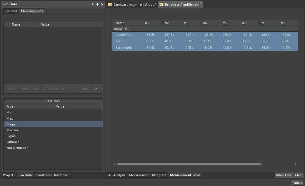
To perform a sensitivity analysis there must be a suitable measurement configured. In the image below, the AC Sweep analysis has an Output Expression set up; dB(v(OUT)), and this output has two measurements configured; BW (short for Bandwidth) and MAX (maximum amplitude). The sensitivity can be calculated for either of these measurements.

To analyze the sensitivity, enable the Sensitivity option in the Simulation Dashboard as shown below, then click the Settings icon to open the Advanced Analysis Settings dialog, where the sensitivity options can be enabled on the Sensitivity tab of the dialog.

If you choose to calculate the Sensitivity, the Temperature Sweep, Sweep and Monte Carlo analyses will not be available.

Configure the Sensitivity settings as required, close the Advanced Analysis Settings dialog and Run the analysis (AC Sweep in this example). When the waveforms appear, the Sim Data panel will also open. Switch to the Measurements tab of the panel, select the required set of measurement results and click the Sensitivity button (as shown below), to switch to the Sensitivity tab of the SDF results window. The sensitivity results are displayed in a table so you can quickly identify the component that has the greatest sensitivity to variations in its value.

The sensitivity results are displayed in a table so you can quickly identify the component that has the greatest sensitivity .

Schematic Design for Simulation

There are several mandatory steps that must be followed in order for the simulation to be successful. It is also essential to perform an electrical rules check of the circuit before running the simulation.

If all design rules and required conditions are met, the Simulation Dashboard will display green tick icons to notify you verification has been successful. When the schematic sheet is active use the Simulate » Simulation Dashboard command to open the Simulation Dashboard.

This schematic has been verified and is now ready to be simulated.

Conditions Required for Simulation

The necessary conditions for the design of the electrical circuit are as follows:

1. The schematic used in the simulation must be part of a project (*.PrjPcb). If the schematic sheet has been created without being linked to a project, the simulation command in the Simulate menu will be inactive. The ability to work with the Simulation Dashboard is also restricted, as shown below.

Simulation is not available for a schematic that is not part of a project.

2. There should be at least one voltage or current source, or signal source, as part of the schematic design. If there is no source, the simulation can still be performed and you will be warned by the message Need to add source in the Preparation section of the Simulation Dashboard. For a detailed description of the sources and how to place them, refer to the Signal Sources section.

Need to add source notification.

3. The schematic must include a GND net, that is, it must contain a node with a potential of zero that the simulation engine can use as a reference node. The simulation will not continue without this condition. The Verification section of the Simulation Dashboard displays a warning if this error is present. The Details link redirects you to the Messages panel for more information.

No reference node notification.

In the Active Bar there are commands to place a GND node, along with other power ports of different values, style and purpose.

A GND node (and other power ports) can be placed from the Active Bar.

4. In addition to the mandatory conditions for the schematic, there must also be a valid model for every component. Components placed from the supplied simulation-specific libraries include a suitable model. Components that have been placed from your own libraries will need to have a model added, either in the schematic library editor, or directly on the schematic.

If a component is missing a model, a warning will appear in the Verification section of the Simulation Dashboard. A similar warning will also appear when there is an error in the model.

Components without Models notification.

Resolving Model Errors

You have a choice how to solve such errors if they occur:

• For basis R, L, C components, the information field at the top of the Simulation Dashboard will prompt to add the missing models automatically. Click the Assign link to perform this automatic action.
• Alternatively, each component that is missing a model will be listed in the Simulation Dashboard, as shown for R1 in the image above. Click the +Add Model link to add the model manually. This will redirect you to the Sim Model dialog, where you can manually select and add a model to the chosen component. The process of adding a simulation model to a component is described in detail in the Adding models to the schematic components section.

While working on the schematic structure and the parameters of the components, there is a need to repeatedly check the design. Changes made to the schematics automatically trigger repeated checks, if errors are detected you will be notified with a corresponding message. If the verification is successful, this procedure is invisible to the user and so does not distract you from your work.

When simulating an electrical circuit, assigning a net name is not a mandatory condition but we recommend it for convenience. Assigning a net name makes the selection of points for displaying characteristics clearer, especially when working with complex schematics. In the Simulation Dashboard, for some types of calculations it is possible to select the desired points to display the characteristics on the plots in the Output Expression sections, if you have identified those points with a net label.

Select the required Output Expressions.

You can place a Net Label from the Active Bar, or via the Place » Net Label menu command. Before placing the Net Label on the schematic press the Tab keyboard shortcut to open the Properties panel, where you can define the Net Name.

Net Label placement command.

Adding Models to the Schematic Components

Components and models can be stored as discrete files, or they can be stored in an Altium Workspace, such as Altium 365. Let's review how you do that with file-based components and models first.

Working with File-based Libraries and Models

In order to use file-based libraries and model files, they must be installed. To do this, open the Operations menu in the Components panel and select the File-based Libraries Preferences command to open the Available File-based Libraries dialog, here you add local libraries and models to the Components panel for access.

Open the Available File-based Libraries dialog.

Use the Add Library button on the Installed tab to select the desired local files, as shown below. As with any installed library, the order the libraries and models are listed dictates the order they are used by the software. Use the Move Up and Move Down buttons to change the order.

An example of libraries and model files being installed.

Placing a Simulation-ready Component

To place a component on a schematic from any local or cloud library, you can:

• Use the Place command from the right-click context menu
• Double-click on the component in the panel
• Drag the component from the panel into an open document

Right-click on the component and select the Place command.

If you are working with a library that has some components with simulation models and some without, enable the Simulation column in the Components panel to make it easy to locate the simulation-ready components. To do this, right-click on one of the current column headings in the Components panel and choose Select Columns from the context menu, then enable the Simulation column in the Select columns dialog.

Enable the Simulation column to quickly identify which components have simulation models.
You can also examine the simulation model details in the Component Details section of the panel.

If a library component has a simulation model attached, you can examine the model in the Component Details section of the Components panel, as shown in the image above.

Placing a Component when you only have the Model

If you have a simulation model but do not have a component to add it to, you can actually place the model file instead. When you do this, the software analyzes the model and locates a suitable symbol in the Simulation Generic Components library. Discrete components will have a symbol that suits that type of component, components that are modeled by a subcircuit will have a simple rectangular symbol.

You can place a model directly on the schematic, the software will generate a suitable symbol.

The table below lists the supported model-kinds and the Simulation Generic Components library component symbol that is placed.

Component	Model Text	Symbol (SIM Library Design Item ID)
Resistor	.MODEL <model name> RES	Resistor
Capacitor	.MODEL <model name> CAP	Capacitor
Inductor	.MODEL <model name> IND	Inductor
Diode	.MODEL <model name> D	Diode
Bipolar transistor	.MODEL <model name> NPN	BJT NPN 4 MGP
Bipolar transistor	.MODEL <model name> PNP	BJT PNP 4 MGP
Junction FET	.MODEL <model name> NJF	JFET N-ch Level2
Junction FET	.MODEL <model name> PJF	JFET P-ch Level2
MOSFET	.MODEL <model name> NMOS	MOSFET N-ch Level1
MOSFET	.MODEL <model name> PMOS	MOSFET P-ch Level1

Placing a Simulation-Ready Component from the Manufacturer Part Search Panel

The Manufacturing Part Search Panel gives designers access to millions of components from thousands of component manufacturers. The panel includes power parametric filtering, including a filter to only display components that include a simulation model. When this filter is applied, only components that include a simulation model, will be displayed.

The Manufacturer Part Search panel gives access to millions of components, some that include simulation models.

At the moment, the simulation models do not have the model pin definitions mapped to the physical component pins. Because this mapping is not defined, the software will apply default 1 to 1 mapping (model pin 1 maps to physical pin 1). Because of this the mapping may be incorrect, if you use one of these components you simulation will either fail or not function correctly.

To help with this, the simulator includes an option that, when enabled, automatically replaces the existing component symbol with a generic component symbol. This generic component symbol is a simple rectangle that is created during placement, whose pins that are automatically mapped to the correct model pins. To use this feature, enable the the Always Generate Model Symbol for Manufacturer Part Search Panel Using Simulation Model Description option to the Simulation - General page of the Preferences dialog.

Enable the Always Generate Model Symbol option if you use simulation-ready components from the Manufacturer Part Search panel.

Adding a Model to a Placed Component

To view the models that have been attached to a placed component, use the Properties panel. The existing models are specified in the Parameters section of the panel, when the option has been enabled.

To add a simulation model to the component, click the Add button at the bottom of the Parameters section, and choose Simulation from the menu that appears.

Existing component models can be viewed/edited and new models attached in the Properties panel.

The Sim Model dialog will open. Model selection and schematic symbol pin to model pin mappings are performed in this dialog.

Select a simulation model and map its pin definitions to the schematic symbol pins, in the Sim Model dialog.

Choose the Source of the Model

Before clicking the Browse button to choose the model, click to set the required Source mode. The Source button that you enable determines what will happen when the Browse button is clicked:

• Local - use this option to browse for a model file stored locally on a local hard drive or network server.
• Library - use this option to browse for a model that has been made available through the Available File-based Libraries dialog, as described previously in the Working with File-based Libraries and Models section.
• Server - use this option to browse for a model located in a connected Altium Workspace.
• Octopart - use this option to browse for a component model available in the Manufacturer Part Search dialog (this dialog is the same as the Manufacturer Part Search panel). Enable the Filter section of the dialog (), then search and enable the Has Simulation filter so that only components that include a simulation model are returned. Then use the main search field to search and see if the component model you require is available (show image). Although the Manufacturer Part Search panel returns complete components, only the simulation model of the chosen component will be used in your design.

Browse and Select the Model

Once you have selected the Source, click the Browse button to choose the model file. The dialogs that appear and the approach that you use to locate the model, depends on which Source option you enabled. The slides below show the different dialog that opens for each of the four Source modes:

The slides show the different dialog that appears for each of the four Source modes.

After selecting the model file, an indication of compatibility and operability of the model is the display of the text, parameters and information that is included in the model file. This information appears in the Model Description region of the Sim Model dialog. Switch to the Model File tab to examine the content of the model.

It is also important to confirm that the model Format Type option is correctly set. The software will attempt to detect and assign this automatically, confirm that it is correct.

Mapping the Model Pins to the Component Symbol Pins

For correct model operation it is necessary to check the association between the component pins and the model pins, because they may not map one-to-one. Most model files include a description of the model pin numbers in the text of the model file, as shown in the image below, use this to map each model pin to the correct symbol pin.

Each component pin must be mapped to the corresponding model pin.

Creating a new Model File

Some models are provided by manufacturers and suppliers as downloadable text files. Sometimes the model detail is presented as text on a web page instead of a download file, in this situation you can create a new model file in Altium NEXUS and copy/paste the content from the web page into your new model file. Use the relevant command in the File » New » Mixed Simulation sub-menu, as shown below.

Commands to create a new, empty model file.

You can then Copy / Paste the model file information into the model editor.

Example text content of a simulation model.

Attaching a Model in the Library Editor

As well as attaching a model to the component symbol that has been placed on the schematic, you can also attach the model to the component in the schematic library editor.

This is performed in the schematic library editor. The models that are attached to the component are listed below the graphical editing section, for the selected component. Click the Add Simulation button to add a simulation model.

Attaching a simulation model to a library component.

The Sim Model dialog will open, select the Source location of the model to add to the component and click the Browse button.

Set the model Source location, then browse to locate the model.

Note that the model must be installed in the Components panel or be a part of the active project in order to be displayed in the list of available models.

Browse and locate the required model.

The Model Name and Location of the model file will be specified in the relevant fields, and the model detail will display in the Model File tab on the right side of the dialog. Click the OK button to add the model to the library component.

The created model has been attached to the component in the library editor, hover the cursor over the image to show the model details.

The new simulation model will be displayed in the section below the graphical editing window after attaching it to the symbol. Save the changes you have made.

Save the component after attaching the model.

Working with Workspace Components and Models

You can use all of your existing libraries when working with the circuit simulator, including Workspace libraries, which can also have simulation models attached. You can view the availability of the model in a particular component in the Components panel in the Details section. To learn more about Workspace components, refer to the Quick Guide to Component Management with a Workspace.

Workspace components differ from file-based components. In a file-based component the symbol is the core element; it holds the parameters, with the footprint and simulation model being attached to it.

In a Workspace component, the component item holds the parameters and brings the other elements together; including the symbol, the footprint, and the simulation model. Each of the elements is stored as a separate item in the Workspace. When you add a simulation model to an existing Workspace component, you must first upload the model to the Workspace, and then attach it to the Workspace component. The simulation model can be uploaded separately, or it can uploaded as part of the process of attaching it to the component.

This difference between file-based and Workspace components means there is a slightly different approach to editing a Workspace component.

Editing the Workspace Component

The easiest way to edit an existing Workspace component and add a simulation model to it, is to locate the component in the Components panel, then right-click and select Edit from the context menu, as shown below. The component will open for editing in the Component Editor.

Right-click on the Workspace component to Edit it.

Adding a Simulation Model to the Component

To add a simulation model to the component, visually locate the Add Simulation controls, click the dropdown, and select the New option, as shown below.

Adding a new simulation model to the component.

The Existing command opens a list of models already available in the Workspace. The New command creates a new, empty model item which opens in a new document tab, from where you can select the file-based simulation model that you want to add.

Browse to select the simulation model, the content of the model you select will be copied into the newly created simulation model item.

To add a new simulation model, click the Browse button. The Browse Libraries dialog will open, where you can select from the list of currently installed libraries/models. If the model has not been installed in the software, click the ellipsis () button in the Browse Libraries dialog to open the Available File-based Libraries dialog, where you can Install additional libraries and models. To learn more about installing libraries and models, refer to the Working with File-based Libraries and Models section earlier in this guide.

Locate the required model in the Browse Libraries dialog, click the ellipsis if you need to install additional models.

Once you have chosen the model in the Browse Libraries dialog, click OK. Save the simulation model item, then close it (right-click on its document tab to close it). Your view will return to the Workspace Component Editor.

Saving the Updated Workspace Component

The component now has a simulation model attached, as shown below. The last step is to save the updated component back into the Workspace - this action is referred to as Save to Server. Select the Save to Server command in the File menu. When you select the command the component is validated, and then the Edit Revision dialog opens where you can enter optional release notes about the changes made in this new revision of the component. When the process of saving the new revision of the component is complete, the component is automatically closed.

The Workspace component is now ready to be used for simulation in your design.

Use the Save to Server command to update the component in the Workspace.

If the Workspace component has already been placed on the schematic, it can be updated to the latest revision by clicking the Update to the Latest Revsion button, as shown below.

Components that have already been placed from the Workspace can be updated to the latest revsion if they become out of date.

If the component has not yet been placed from the Components panel, confirm that the new simulation model is displayed in the Models section of the panel before placing it. If the simulation model is not displayed, right-click in the component list section of the Components panel and select Refresh to update the local cache.

The simulation model has been added to the Workspace component. Right-click to Refresh if the sim model details do not display.

Simulation, finding the Balance between Accuracy and Performance

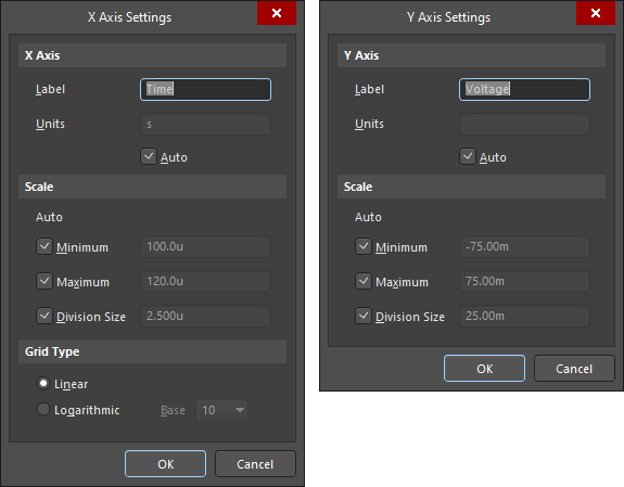
An important part of the simulation setup is setting the correct values for the ranges used for the simulation.

For example, the defaults may not match the required simulation time needed, based on the circuit’s characteristics. As an example, consider a transient characteristic configured with a From - To time interval from 0 to 1u, as shown below.

The Transient time interval has been configured from 0 to 1u.

In this circuit, the source has been configured to have a Period of 1uS, as shown below.

The period of the source is 1u.

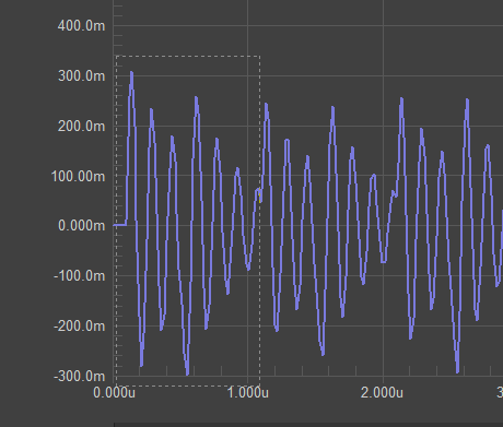
This Transient range will not allow the circuit to properly simulate given the characteristics of the circuit’s operation, as shown below.

The Transient time range is too short for the Period configured in the source.

Similarly, when the range is wide (for example 0 - 100u), it will also be difficult to analyze the plot, and the time required for the analysis also increases.

The Transient time range is too wide.

Instead, choose a range value greater than the signal period value, for example, 5 periods (0 - 5u). This should be sufficient for the circuit to become stable, but not excessive for this type of calculation.

A suitable time range for a Transient analysis of this circuit.

It is also important to consider selecting a proportional step of values for the calculation or the number of points displayed on the plot. If you select an excessive number of points, the calculation will be slower, and an insufficient number of points will result in inaccurate calculations.

For example, consider the amplitude-frequency characteristics shown below, the first configured to use 10 points, the second configured to use 1000 points. The difference in the number of points used does not make a considerable difference in the calculation time, but significantly increases the accuracy of characteristics.

The analysis results when an insufficient number of points has been used for the calculation.

A suitable number of points has been used for the calculation.

Results Display and Analysis

The results of each type of calculation display on a named tab in the SDF window that opens whenever a simulation is performed. When all the calculations are run together (press F9, or select the Simulate » Run Simulation command), you can switch between plots by clicking the tab at the bottom of the open SDF document.

Each analysis type is displayed on a named tab in the SDF file.

Simulation results can be saved if you wish to view and edit them later. Right-click on the document tab at the top of the Workspace and select the Save command. If you plan to run different types of analyses and save each SDF file, use the File » Save As command instead so that each SDF file can be given a unique name.

The SDF file can be saved via the right-click context menu.

All saved simulation results are displayed in the Simulation Dashboard in the Results section. To reopen a specific plot, click the ellipsis and select Show Results from the menu, or double-click on the analysis name. The menu can also be used to Edit the chart Title and Description, restore the settings of the plot in the Analysis Setup & Run area (Load Profile), and Delete those results.

The simulation Results for each analysis type that has been run, can be accessed in the Simulation Dashboard.

You can also lock the results of a particular simulation. If you do, the next simulation of the same type will be saved as a new Result with a sequential numerical suffix appended to the name.

Click the Lock icon to save a specific version of the calculation.

Working with Plots

The image below shows the names of the various elements in the result waveforms.

Understanding the different elements in the simulation results.

Quick tips for working in the waveform window:

• A wave can be moved from one plot to another by clicking holding on the waveform name, then dragging it to a different plot.
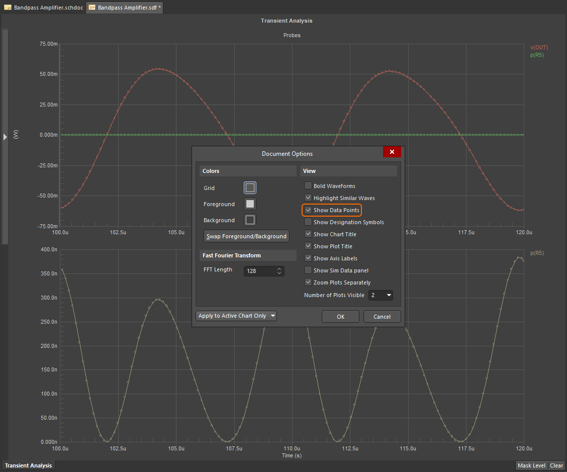
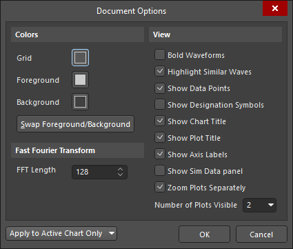
• To display an existing wave on a new, separate plot, double-click on the name, then in the Edit Waveform dialog select New Plot in the Plot Number dropdown (show image). After doing this you may need to change the number of visible plots, this is done in the Document Options dialog (Tools menu).
• Double-click anywhere within a plot to open the Plot Options dialog, where you can configure the Title, Grid Lines, and Line Style. (show image)
• Double-click on an axis to label and configure that axis. (show image)
• Double-click on the chart title to open the Chart Options dialog, where you can name the chart and also configure which cursor measurements are displayed on that plot, if the cursors are currently enabled. (show image)
• To zoom in to examine an area of a plot, left-click-and-drag a rectangle to define the new view area. To restore the view, right-click and select Fit Document. (show image)
• Select Tools » Document Options from the menu to open the Document Options dialog, where you can configure the colors, the visibility of various wave, chart and plot elements (including the data points), and define the FFT length. (show image)

We will use the early characteristic of the transient process and the image of the signal at the source output to demonstrate how to work with plots.

The transient process characteristic and the signal at the source output.

Left-click in the legend to select one of the signals on the plot, click a second time to de-select it.

Click once on a signal name to select. Click again to de-select it.

Right mouse click on a signal name to open a menu with a set of commands for editing the selected signal, as shown below.

Menu of commands available for the selected signal.

Measurement Cursors

It is possible to set two cursors simultaneously and move them along the X-axis. The coordinates of the intersection of the cursor and the plot are displayed in the lower part of the window. Measurement details can also be displayed below the plot, right-click on the plot and select Chart Options to configure this.

Use the right-click Cursor Off command to remove a cursor.

Example of using cursors.

The cursors can also be used to perform various measurements on the waveforms, open the Sim Data panel to display the measurements calculated from the current locations of the two cursors.

The cursors can be used to perform measurements from the waveform. Measurement results are displayed in the Sim Data panel.

You can edit an already displayed signal by selecting the Edit Wave command from the right-click menu (or double-click on the signal name). This will open the Edit Waveform dialog.

Select the Edit Wave command to open the Edit Waveform dialog.

Defining a Mathematical Expression

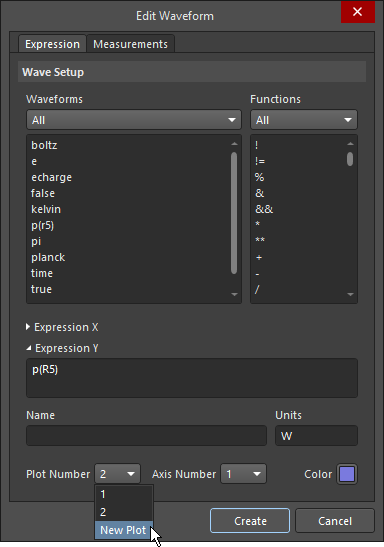
As well as allowing you to select the Waveform to be observed, the Edit Waveform dialog can be used to define a mathematical Expression.

Build an Expression by selecting the Waveform (it will be included in the Expression field when you click on it in the Waveforms list), apply the required Function, then continue to select Waveforms to build up the required Expression. Use the Name field to give your Expression a meaningful name. In addition, you can change Units and the Color of the displayed waveform.

Create your own output expressions.

If you right-click anywhere on the plots (other than on a waveform name), a menu of commands appears, where you can: add a waveform to an existing plot (Add Wave to Plot); add an additional plot (Add Plot); delete a plot (Delete Plot); configure various options; and restore the view of the plots (Fit Document). Use this command if you have zoomed in to a small area of a plot to examine it in detail.

Adding a New Plot

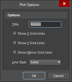
New plots are added via the Plot Wizard. The sequence of steps and the result is shown in the images below.

Right-click and select Add Plot to launch the Wizard, then name it and configure the grids.

Click Add to select a waveform from the available waveforms.

The new plot of v(out) has been added to the chart.

What is a SPICE netlist and how to read it?

The SPICE netlist is a textual representation of the circuit. It must include all necessary components with parameters, component models, connections, and types of analysis. It is the SPICE netlist that is processed by the simulation engine. The graphical representation of the schematic is used to simplify the creation of the netlist from the user's work when simulating. Because the netlist is created automatically when designing the schematic there is no need to manually create it, simplifying the process and reducing potential errors.

The specification of components and connections requires a special syntax to describe the circuit. Despite the complexity of the method it has its advantages, it allows you to work directly with and simulate from a netlist, as well as from a schematic.

To generate the simulation netlist from your current schematic, select Simulate » Generate Netlist from the menus. To create a new, empty netlist, select the File » New » Mixed-Signal Simulation » AdvancedSim Netlist command from the menus.

Command to create a netlist.

To understand the content consider the example netlist shown below, that matches the schematic shown beneath it:

• Lines with an "*" at the beginning are comments, used as auxiliary text
• CC11 0 NetC11_2 100nF is the component description, where:
  • CC11 component designation
  • 0 NetC11_2 - nets that the component's pins are connected to, in this example the first pin of the capacitor is connected to the GND (0) circuit, the second to NetC11_2
  • 100nF - component value
• VV6 NetC14_2 0 DC 0 PULSE(0 5 100n 10n 10n 400n 1u) AC 1mV 0 - signal source description:
  • VV6 - component designation
  • NetC14_2 0 - component connection pins
  • DC 0 / AC 1mV / 0 - signal source parameters: DC, AC, phase
  • PULSE(0 5 100n 10n 10n 400n 1u) - output signal parameters: Initial Value, Pulsed Value, Time Delay, Rise Time, Fall Time, Pulse Width, Period
• .PRINT =1 NetC13_1 NetC14_2 - command to show signals in the form of a plot
• *Selected Circuit Analyses:
  • .TRAN 1 10u 0 1 - selected type of calculation (transient calculation) and calculation parameters (start time, end time, step)
• *Models and Subcircuits:
  • .model PMOSFET_Level1 pmos (Level=1) - link to the transistor model used
• .END - end of document

Example netlist.

The schematic that the netlist was generated from.

To run a simulation directly from an open netlist, select Simulate » Run (or press the F9 hotkey).

You can run a simulation directly from the netlist.

The simulation result is the same as the one obtained earlier using the schematic and the Simulation Dashboard panel.

The results after simulating directly from the netlist.

Simulation Troubleshooting

When a circuit will not simulate you must identify if the problem is in the circuit, or the process of simulation. Follow the information contained in this section of the reference and work through the suggested points, trying one at a time.

Sometimes during a simulation, a message will be displayed reporting errors or warnings. These messages are listed in the Messages panel.

Warning Messages - Warning messages are not fatal to the simulation. They generally provide information about changes that SPICE had to make to the circuit in order to complete the simulation. These include invalid or missing parameters, and so on.

Error Messages - Error messages provide information about problems that the Mixed Simulator could not resolve and were fatal to the simulation process. Error messages indicate that simulation results could not be generated, so they must be corrected before you will be able to analyze the circuit.

Trouble-shooting simulation analysis failures

One of the challenges of all Simulators is convergence. What exactly is meant by the term, convergence? Like most Simulators, the Mixed Simulator's SPICE engine uses an iterative process of repeatedly solving the equations that represent your circuit, to find the quiescent circuit voltages and currents. If it fails to find these voltages and current (fails to converge) then it will not be able to perform an analysis of the circuit.

SPICE uses simultaneous linear equations, expressed in matrix form, to determine the operating point (DC voltages and currents) of a circuit at each step of the simulation. The circuit is reduced to an array of conductances which are placed in the matrix to form the equations (G * V = I). When a circuit includes nonlinear elements, SPICE uses multiple iterations of the linear equations to account for the non-linearities. SPICE makes an initial guess at the node voltages then calculates the branch currents based on the conductances in the circuit. SPICE then uses the branch currents to recalculate the node voltages, and the cycle is repeated. This cycle continues until all of the node voltages and branch currents fall within specified tolerances (converge).

However, if the voltages or currents do not converge within a specified number of iterations, SPICE produces error messages (such as singular matrix, Gmin stepping failed, source stepping failed or iteration limit reached) and aborts the simulation. SPICE uses the results of each simulation step as the initial guesses for the next step. If you are performing a Transient analysis (that is, time is being stepped) and SPICE cannot converge on a solution using the specified timestep, the timestep is automatically reduced, and the cycle is repeated. If the timestep is reduced too far, SPICE displays a Timestep too small message and aborts the simulation.

General simulation convergence troubleshooting

When a simulation analysis fails, the most common problem is failure of the circuit to converge to a sensible operating point. Use the following techniques to solve convergence problems.

Convergence troubleshooting steps

• When you have a convergence problem, first turn off all the analyses except the Operating Point analysis.
• Consult the Messages panel for any errors/warnings relating to simulation.
• Make sure the circuit is wired correctly. Dangling nodes and stray parts are not allowed.
• Ensure that the circuit has a ground node, and that every node in the circuit has a DC path to this ground. Components that can isolate a node include transformers and capacitors. Voltage sources are considered a DC short circuit, current sources are considered a DC open circuit.
• Ensure that zeros have not been confused with the letter O when entering simulation parameters.
• Ensure that proper SPICE multipliers have been specified (MEG instead of M for 1E+6) for any component values or simulation parameters. Multipliers are not case sensitive. Also, spaces between values and multipliers are not allowed. For example it should be 1.0uF, not 1.0 uF.
• Make sure all devices and sources are set to their proper values.
• Make sure the gain of any dependent source is correctly set.
• Temporarily eliminate series capacitors or current sources and re-run the simulation.
• Temporarily eliminate parallel inductors or voltage sources and re-run the simulation.
• On the Advanced tab of the Advanced Analysis Settings dialog (click  in the Analysis Setup & Run section of the Simulation Dashboard), increase the value of the ITL1 parameter to 300. This will allow the Operating Point analysis to go through more iterations before giving up.
• On the Advanced tab of the Advanced Analysis Settings dialog, set the value of the RSHUNT1. This value of resistance is added between each circuit node and the ground helps to correct problems such as "singular matrix" errors. As a rule, the RSHUNT value must be set to a very high resistance, such as 1e12.
• Add .NS (Nodeset) devices to define the node voltages. If the initial guess of a node voltage is way off, the Nodeset device can be used to predefine a starting voltage that is used for a preliminary pass of the operating point analysis. Configure the Initial Voltage parameter in each Nodeset device that you place. A Nodeset can be placed from the Simulation Generic Components library, or the Simulation Sources library. If the Nodeset device is placed from the Simulation Sources library, the Initial Voltage parameter will not be visible by default. To resolve this, select the component to display its settings in the Properties panel, select the Simulation model in the panel, and click the  button to open the Sim Model dialog. The parameter will be listed on the right hand side of the dialog, enable the Show in Component checkbox to display it in the Properties panel, where it can easily be examined and edited. If you do not see it in the Properties panel, click the Show More link to display all parameters, then click the  icon to always display it.
• If the Nodeset device does not assist in convergence, try defining the initial conditions by placing .IC devices. In this case the node voltages are held at the specified values during the Operating Point analysis, then released during the Transient analysis. Initial Condition devices can be placed from the same libraries as a Nodeset device, the Initial Voltage parameter must be configured in the same way.
• Enable the Use Initial Conditions option in the Transient settings in the Analysis Setup & Run section of the Simulation Dashboard. This option works in conjunction with the .IC devices (or the IC parameter of the components). By setting this option, the Operating Point analysis is not performed and the specified voltages are used as the initial conditions for the Transient analysis.
• Specify the series resistance parameters of your models and increase the GMIN option (Advanced tab of the Advanced Analysis Settings dialog) by a factor of 10.
• Specify the initial condition (Starting Condition) of semiconductor devices, especially diodes, as OFF. This can help solve numerical convergence problems by skipping the diode (or semiconductor device) for the first iteration, helping improve convergence.

DC Sweep Analysis troubleshooting

When you have a problem with a DC Sweep analysis, first try the steps listed above in the Convergence troubleshooting steps. If you still encounter problems, try the following:

• Change the value of the Primary Step parameter in the Analysis Setup & Run section of the Simulation Dashboard. If discontinuities exist in a device model (perhaps between the linear and saturation regions of the model), increasing the step size may allow the simulation to step over the discontinuity. Making the steps smaller, on the other hand, will allow the simulation to resolve rapid voltage-transition discontinuities.
• Do not use the DC Sweep analysis. Some problems (such as hysteresis) cannot be resolved by DC analysis. In such cases, it is more effective to use the Transient analysis and ramp the values of the appropriate power sources.

Transient Analysis troubleshooting

When you have a problem with a Transient analysis, first try the steps listed above in the Convergence troubleshooting steps. If you still encounter problems, try the following.

On the Advanced tab of the Advanced Analysis Settings dialog (click  in the Analysis Setup & Run section of the Simulation Dashboard):

• Set the RELTOL parameter to 0.01. By increasing the tolerance from its default of 0.001 (0.1% accuracy), fewer iterations will be required to converge on a solution and the simulation will complete much more quickly.
• Increase the value of the ITL4 parameter to 100. This will allow the Transient analysis to go through more iterations for each timestep before giving up. Raising this value may help to eliminate timestep too small errors improving both convergence and simulation speed.
• Reduce the accuracy by increasing the values of ABSTOL and VNTOL, if current/voltage levels allow. Your particular circuit may not require resolutions down to 1uV or 1pA. You should, however, allow at least an order of magnitude below the lowest expected voltage or current levels of your circuit.
• Change the Integration Method to one of the Gear methods. Gear integration requires a longer simulation time, but is generally more stable than trapezoidal. Gear integration may be particularly useful with circuits that oscillate or have feedback paths.

Additional things to try:

• Realistically model your circuit. Add realistic parasitics, especially stray/junction capacitance. Use RC snubbers around diodes. Replace device models with subcircuits, especially for RF and power devices.
• Increase the rise/fall times of any Periodic Pulse sources in your circuit. Even the best pulse generators cannot switch instantaneously.